I want to be clear, I am not an expert, in either cybersecurity or data science. I am interested in both fields so it becomes very fun exploring the intersection.

If you just want the code, click here.

Overview

Introduction
What Are Adversarial Attacks
Applying to recent CTF challenges
Conclusion

Introduction

Adversarial attacks are not new, but they are not a usual category in CTF competitions. With the past year or so, I started seeing more competitions including data science related challenges. I want some spend time to explore some adversarial methods and apply them in examples that are easy to translate for competitions.

Before diving into the main topic, I want to mention that I will assume some understanding of machine learning basics. Maybe in the future I can further explore these basics to build a ground-up understanding.

In this article we will explore white-box model adversarial image attacks and try minimize the difference between the pixels on initial image and the adversarial examples we will create.

What are Adversarial Attacks?

In machine learning, adversarial attacks are techiques that aim to deceive or compromoise an AI system. The techiques can include different types of attacks that specially manipluate the system's input, training data or even the inner workings of the model itself. I will focus on the most on attacks that manipluate the AI system's input to get it to an unintended output. Though you can explore more about adversarial attacks here.

No model is perfect. Machine learning tries to estimate output signals from the training data that is given to it. Models predict an outcome, and in most settings, they usually do a pretty good job at it. There are always inaccuracies but they can accumulate from the dataset, training methods/architecture or they are inherit to the problem itself.

With convolutional neural networks, especially for image-related problems, a model can become good at identifying shapes & edges for classification. Modern image models rely on many parameters (on the smaller end, resnet18 has ~11m parameters) and current research tries to apply these models to bigger and bigger problems.

Exploring adversarial attacks unveils the vulnerability of these seemingly robust models. Despite their sophistication, they can be targeted to produce specific output with a specially crafted input. In this article, we will go through several popular types of attacks and apply our learning to challenges from recent cybersecurity CTF competitions.

Lets try it out

Let's consider the scenario of generating an adversarial example for an ImageNet-trained ResNet18 model. We will try out some different methods to generate adversarial examples starting from an initial image $x$ .

Three examples of model input to ResNet18 Model, an all white image, an all black image, and noise image

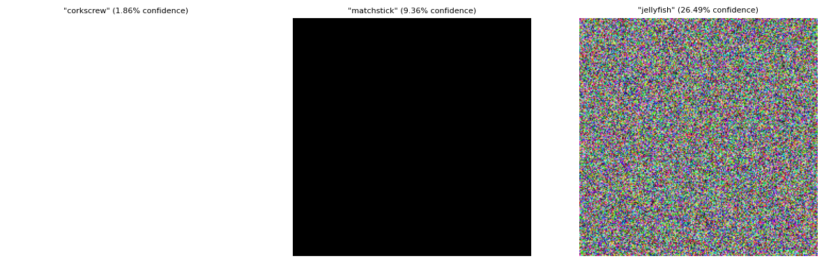
ImageNet-trained ResNet18 model's output probabilities for a white, black and nosie image.

In all three of the solutions, I will only focus on the following cost function that optimizes for the cross-entropy loss over a specific target, $y_{\text{target}}$ .

$\mathcal{L}_{\text{targeted}}(x, y_{\text{target}}) = \text{CE}(y_{\text{target}}, f(x))$

Where:

$x$ denotes the model's input, any image.
$y_{\text{target}}$ is the target class that we want to generate an adversarial example for.
$\text{CE}$ is the Cross Entropy loss function.
$f(x)$ denotes the model.

If we need to, we can also optimize the $\text{CE}$ loss by maximizing the loss of the true label of $x$ and the model's output.

$\mathcal{L}_{\text{untargeted}}(x, y_{\text{true}}) = - \text{CE}(y_{\text{true}}, f(x))$

Where:

$y_{\text{true}}$ is the label we want to optimize against.

For the solutions, we will also try to keep the adversarial example close to the initial image. This means that the difference pixels of the original and adversarial image are within a certain number of pixels. We will do this by clamping the changes after generating an adversarial example or during each iteration. Each solution can just easily remove this restriction, we are keeping it as it leads to the CTF problems easier.

Lastly, these solutions require input to start with, the initial $x^{0}$ . We will start with using the white image from the diagram above, and later transition the attack to use a picture of my bird below.

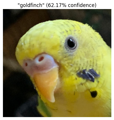
ImageNet-trained ResNet18 model's output probabilities for the bird.

Let's finally jump in the solutions.

Iterative naive solution

We can write out a simple solution to generate an adversarial image given an inital image $x$ . We can iteratively optimize for a better solution.

$x^{(k+1)} = x^{(k)} - \alpha \cdot \nabla_{x^{(k)}} \mathcal{L}_{\text{targeted}}(f(x^{(k)}), y_{\text{target}})$

Where:

$x^{(k)}$ denotes the image at iteration $k$ .
$\alpha$ is the step size at each iteration.
$\nabla_{x^{(k)}} \mathcal{L}_{\text{targeted}}(f(x^{(k)}), y_{\text{target}})$ represents the gradient of the cost function with respect to $x^{(k)}$ .

Using gradient descent, we can slowly come up with a solution that maximizes the probability of the target.

Lets try an example in python using pytorch and apply this simple iterative solution. Starting from a completely white image, lets try to get the model to predict class index $0$ , which maps to "tench." Here is the python code to do this gradient descent:

target_output = torch.tensor([0], dtype=torch.long) # class 0 is "tench"

# convert the white image to a tensor and normalize it to the same range as the model's input (0-1)
x = torch.tensor(white_img, dtype=torch.float32).permute(2, 0, 1).unsqueeze(0) / 255.0
x.requires_grad = True # allow gradients to be calculated since we want to optimize the image

alpha = 1. # step size for the gradient descent

for iteration in range(15):
    output = model(x)

    # our objective is to maximize the probability of the target class
    loss = F.cross_entropy(output, target_output)

    # calculate the gradient of the loss with respect to the input image
    loss.backward()

    # apply gradient descent to the image, this step is usually done by the optimizer
    # but we're doing it manually here, by taking the gradient of the image and updating it
    x.data = x.data - alpha * x.grad

    # zero the gradient for the next iteration
    x.grad.zero_() # probably not needed

    # clamp the image to the valid pixel range [0, 1]
    x.data = torch.clamp(x.data, 0, 1)

full code: https://github.com/OutWrest/blog-handouts/blob/main/exploring-attacks-1/attacks-introduction.ipynb

Output:

Iter: 0  | Loss:  7.5425 | Pred: "window shade" (5.05% confidence)
Iter: 1  | Loss:  9.2704 | Pred: "dishrag" (3.04% confidence)
Iter: 2  | Loss:  10.1515 | Pred: "nematode" (1.45% confidence)
Iter: 3  | Loss:  7.6952 | Pred: "brain coral" (2.15% confidence)
Iter: 4  | Loss:  5.4389 | Pred: "American alligator" (1.96% confidence)
Iter: 5  | Loss:  4.7709 | Pred: "American alligator" (5.01% confidence)
Iter: 6  | Loss:  3.2306 | Pred: "tench" (10.06% confidence)
Iter: 7  | Loss:  2.2304 | Pred: "brain coral" (17.83% confidence)
Iter: 8  | Loss:  2.4371 | Pred: "tench" (35.66% confidence)
Iter: 9  | Loss:  1.0132 | Pred: "tench" (96.03% confidence)
Iter: 10 | Loss:  0.0390 | Pred: "tench" (99.90% confidence)
Iter: 11 | Loss:  0.0015 | Pred: "tench" (99.92% confidence)
Iter: 12 | Loss:  0.0013 | Pred: "tench" (99.93% confidence)
Iter: 13 | Loss:  0.0012 | Pred: "tench" (99.93% confidence)
Iter: 14 | Loss:  0.0011 | Pred: "tench" (99.94% confidence)

"tench" maps to our target index of $0$ , succes!

Lets see how the adversarial example looks.

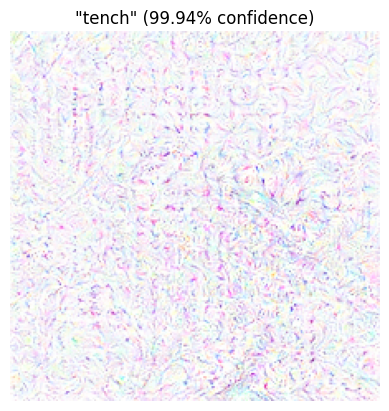
The output adversarial example.

Starting from a completely white image - we are able to produce an adversarial image with any class we pick. The adversarial example is not visually recognizable as a "tench" but the model predicts it with high confidence.

How different is the adversarial example to our original image?

To calculate the difference of the original image adversarial example, we track three different metrics. We will keep track of the max, mean, and min pixel difference of the two images.

The code to do this is very simple:

diff = np.abs(white_img - current_img)
max_diff, mean_diff, min_diff = diff.max(), diff.mean(), diff.min()

Here is the pixel difference from our initial solution:

Max  difference:  209.00
Mean difference:  14.36
Min  difference:  0.00

Let's try to create another adversarial using the same method but lets try to minimize our changes to the image. We will clamp the image so that the changes are within a certain range. I will arbitrarily pick that our adversarial example should within $10$ pixels. This is common theme that shows up in CTF challeges, so lets try this out here.

Iterative naive solution (with clamping)

Let's define a new function $\text{clip}$ that can simplify clamping.

$\text{clip}(x,\epsilon) = \text{clamp}(x, x - \epsilon, x + \epsilon)$

Where:

$\text{clamp}(x, \text{min\_value}, \text{max\_value})$ is function that clamps the value of $x$ between $\text{min\_value}$ and $\text{max\_value}$ .
$\epsilon$ is the maximum allowed change.

We easily add a restriction to our equation to clip $x^{(k)}$ to be within $10$ pixels of $x^{0}$ .

$x^{(k+1)} = \text{clip}(x^{(k)} - \alpha \cdot \nabla_{x^{(k)}} \mathcal{L}_{\text{targeted}}(f(x^{(k)}), y_{\text{target}}), \epsilon)$

In the arbitrary restriction, we should set $\epsilon = 10$ . Let's write the code out to include this restriction. We will also track the pixel differences during each iteration.

target_output = torch.tensor([0], dtype=torch.long)

white_img_tensor = torch.tensor(white_img, dtype=torch.float32).permute(2, 0, 1).unsqueeze(0) / 255.0

x = torch.tensor(white_img, dtype=torch.float32).permute(2, 0, 1).unsqueeze(0) / 255.0
x.requires_grad = True

# reduced from 1 to 0.1
alpha = 0.1

epsilon = 10. / 255.

for iteration in range(25):
    output = model(x)

    loss = F.cross_entropy(output, target_output)

    model.zero_grad()
    loss.backward()

    x.data = x.data - alpha * x.grad

    x.grad.zero_()
    x.data = torch.clamp(x.data, 0, 1)

    # clamp within epsilon
    x.data = torch.clamp(x.data, white_img_tensor - epsilon, white_img_tensor + epsilon)

full code: https://github.com/OutWrest/blog-handouts/blob/main/exploring-attacks-1/attacks-introduction.ipynb

Output:

Iter: 0  | Loss:  7.5425 | min/max/mean: 0.00/4.00/0.51 | Pred: "corkscrew" (1.76% confidence)
Iter: 1  | Loss:  7.4247 | min/max/mean: 0.00/10.00/0.67 | Pred: "corkscrew" (1.45% confidence)
Iter: 2  | Loss:  7.8976 | min/max/mean: 0.00/10.00/0.88 | Pred: "ski" (1.38% confidence)
Iter: 3  | Loss:  7.8823 | min/max/mean: 0.00/10.00/1.11 | Pred: "ski" (1.74% confidence)
Iter: 4  | Loss:  7.5663 | min/max/mean: 0.00/10.00/1.34 | Pred: "ski" (2.05% confidence)
Iter: 5  | Loss:  6.6579 | min/max/mean: 0.00/10.00/1.57 | Pred: "snowmobile" (2.57% confidence)
Iter: 6  | Loss:  6.3951 | min/max/mean: 0.00/10.00/1.82 | Pred: "envelope" (3.24% confidence)
Iter: 7  | Loss:  6.9340 | min/max/mean: 0.00/10.00/2.11 | Pred: "spider web" (1.73% confidence)
Iter: 8  | Loss:  6.3351 | min/max/mean: 0.00/10.00/2.31 | Pred: "whistle" (4.70% confidence)
Iter: 9  | Loss:  5.5793 | min/max/mean: 0.00/10.00/2.48 | Pred: "spider web" (6.55% confidence)
Iter: 10 | Loss:  5.4742 | min/max/mean: 0.00/10.00/2.64 | Pred: "tray" (10.74% confidence)
Iter: 11 | Loss:  5.0233 | min/max/mean: 0.00/10.00/2.82 | Pred: "spider web" (5.89% confidence)
Iter: 12 | Loss:  4.9147 | min/max/mean: 0.00/10.00/2.95 | Pred: "tray" (4.78% confidence)
Iter: 13 | Loss:  3.1300 | min/max/mean: 0.00/10.00/3.08 | Pred: "envelope" (3.82% confidence)
Iter: 14 | Loss:  4.8309 | min/max/mean: 0.00/10.00/3.23 | Pred: "tench" (5.76% confidence)
Iter: 15 | Loss:  2.7523 | min/max/mean: 0.00/10.00/3.34 | Pred: "brain coral" (8.50% confidence)
Iter: 16 | Loss:  3.3318 | min/max/mean: 0.00/10.00/3.46 | Pred: "tench" (4.90% confidence)
Iter: 17 | Loss:  2.8901 | min/max/mean: 0.00/10.00/3.57 | Pred: "brain coral" (10.10% confidence)
Iter: 18 | Loss:  3.0373 | min/max/mean: 0.00/10.00/3.71 | Pred: "broom" (4.58% confidence)
Iter: 19 | Loss:  3.7803 | min/max/mean: 0.00/10.00/3.83 | Pred: "tench" (30.13% confidence)
Iter: 20 | Loss:  1.1454 | min/max/mean: 0.00/10.00/3.90 | Pred: "tench" (50.96% confidence)
Iter: 21 | Loss:  0.5941 | min/max/mean: 0.00/10.00/3.95 | Pred: "tench" (74.24% confidence)
Iter: 22 | Loss:  0.2818 | min/max/mean: 0.00/10.00/3.99 | Pred: "tench" (99.14% confidence)
Iter: 23 | Loss:  0.0085 | min/max/mean: 0.00/10.00/4.03 | Pred: "tench" (99.76% confidence)
Iter: 24 | Loss:  0.0051 | min/max/mean: 0.00/10.00/4.03 | Pred: "tench" (99.81% confidence)

We needed to do more interations than previous example. but we seem to still be able to create an adversarial example.

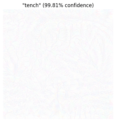
The output adversarial example with clamping.

Applying solution to an actual image

Using the burb example shown earlier in the article, let's try to create an adversarial example that would classified as a assault rifle (index $413$ ). We will also use a lower $\epsilon$ , the perturbations should be within $1$ pixel of the original image.

target_output = torch.tensor([413], dtype=torch.long)

burb_img_tensor = torch.tensor(burb_img, dtype=torch.float32).permute(2, 0, 1).unsqueeze(0) / 255.0

x = torch.tensor(burb_img, dtype=torch.float32).permute(2, 0, 1).unsqueeze(0) / 255.0
x.requires_grad = True

alpha = 0.1

# lets lower the epsilon to a lower pixel difference
epsilon = 1. / 255.

for iteration in range(10):
    output = model(x)

    loss = F.cross_entropy(output, target_output)

    model.zero_grad()
    loss.backward()

    x.data = x.data - alpha * x.grad

    x.grad.zero_()
    x.data = torch.clamp(x.data, 0, 1)
    x.data = torch.clamp(x.data, burb_img_tensor - epsilon, burb_img_tensor + epsilon)

full code: https://github.com/OutWrest/blog-handouts/blob/main/exploring-attacks-1/attacks-introduction.ipynb

Output:

Iter: 0  | Loss:  13.438 | min/max/mean: 0.00/2.00/0.76 | Pred: "puffer" (5.17% confidence)
Iter: 1  | Loss:  8.1450 | min/max/mean: 0.00/2.00/0.70 | Pred: "goose" (6.03% confidence)
Iter: 2  | Loss:  4.7022 | min/max/mean: 0.00/2.00/0.73 | Pred: "assault rifle" (4.97% confidence)
Iter: 3  | Loss:  2.8506 | min/max/mean: 0.00/2.00/0.75 | Pred: "assault rifle" (15.59% confidence)
Iter: 4  | Loss:  1.6048 | min/max/mean: 0.00/2.00/0.77 | Pred: "assault rifle" (24.72% confidence)
Iter: 5  | Loss:  1.1955 | min/max/mean: 0.00/2.00/0.77 | Pred: "assault rifle" (64.57% confidence)
Iter: 6  | Loss:  0.3494 | min/max/mean: 0.00/2.00/0.71 | Pred: "assault rifle" (88.91% confidence)
Iter: 7  | Loss:  0.0869 | min/max/mean: 0.00/2.00/0.66 | Pred: "assault rifle" (88.80% confidence)
Iter: 8  | Loss:  0.0470 | min/max/mean: 0.00/2.00/0.66 | Pred: "assault rifle" (90.01% confidence)
Iter: 9  | Loss:  0.0376 | min/max/mean: 0.00/2.00/0.66 | Pred: "assault rifle" (91.72% confidence)

Even with a very low $\epsilon$ , we are still able to generate a high confidence image that is able to classified into assault rifle. Let's see what the new image looks like.

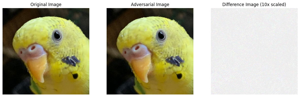
The output adversarial example on burb image.

Following the graident directly is not the best to generate adversarial examples, let's try to implement other methods that are widely used.

Fast Gradient Signed Method (FGSM) Solution

The Fast Gradient Signed Method (FGSM) is a popular technique for generating adversarial examples. It works by calculating the gradient of the loss function with respect to the input image and then perturbing the input image in the direction of the gradient. The amount of perturbation is controlled by a parameter $\epsilon$ .

The adversarial example $x_{\text{adv}}$ is generated as follows:

$x_{\text{adv}} = x + \epsilon \cdot \text{sign}(\nabla_x J(\theta, x, y_{\text{target}}))$

Where:

$x$ is the original input image
$\epsilon$ is the perturbation magnitude (how much to change the original image).
$\nabla_x J(\theta, x, y_{\text{target}})$ is the gradient of the loss function $J$ with respect to $x$ .
$\text{sign}(\cdot)$ denotes the sign function.

Let's try to use FSGM on the same example problem that we've been working on using the burb image as the initial image.

target_output = torch.tensor([0], dtype=torch.long) # we will target index 0, which is "tench, Tinca tinca"

burb_img_tensor = torch.tensor(burb_img, dtype=torch.float32).permute(2, 0, 1).unsqueeze(0) / 255.0

x = torch.tensor(burb_img, dtype=torch.float32).permute(2, 0, 1).unsqueeze(0) / 255.0
x.requires_grad = True

epsilon = 2. / 255.

output = model(x)
loss = -F.cross_entropy(output, target_output)

model.zero_grad()
loss.backward()

grad = x.grad.data

x_adv = x + epsilon * grad.sign()
x_adv = torch.clamp(x_adv, 0, 1)

full code: https://github.com/OutWrest/blog-handouts/blob/main/exploring-attacks-1/attacks-introduction.ipynb

Output:

Loss: -9.0888 | min/max/mean: 0.00/3.00/2.00 | Pred: "tench" (29.52% confidence)

In FSGM, we only generate a single example through the calculation and we do not iterate on our adversarial example.

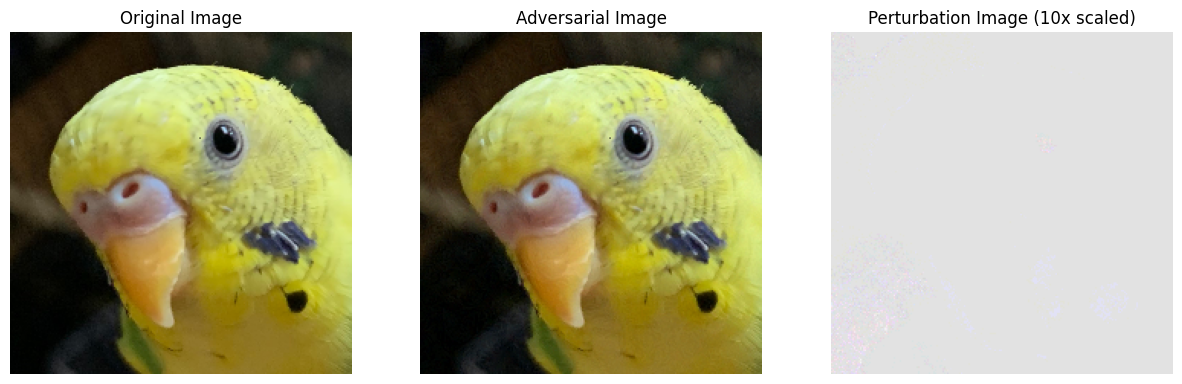
The output adversarial example on burb image using FSGM.

Since FGSM is sensative to epsilon and input image. Depending on input image & target class, it may be that FSGM is the best solution but it is a good start. In our case, we are trying to optimize for very low perturbation to get a model to classify an image into targeted category. While it was able to generate a solution for this case, it did not produce an example with high confidence.

Projected Gradient Descent (PGD) Solution

The Projected Gradient Descent (PGD) method is an iterative extension of FGSM. Instead of applying the perturbation only once, PGD iteratively perturbs the input image in small steps. This iterative process helps to find more effective adversarial examples while keeping the perturbations within a specified limit.

$x^{(k+1)} = \text{clip}(x^{(k)} - \alpha \cdot \text{sign}(\nabla_x J(\theta, x, y_{\text{target}})), \epsilon)$

Where:

$\alpha$ is the step size.
$\epsilon$ is the maximimal allowed perturbation.

Again, let's apply PGD to the same problem.

# we will target index 413, which is "assault rifle, assault gun"
target_output = torch.tensor([413], dtype=torch.long)

burb_img_tensor = torch.tensor(burb_img, dtype=torch.float32).permute(2, 0, 1).unsqueeze(0) / 255.0

x = torch.tensor(burb_img, dtype=torch.float32).permute(2, 0, 1).unsqueeze(0) / 255.0
x.requires_grad = True

epsilon =   5. / 255. # we will allow a maximum of 5 pixel difference
alpha =     1. / 255. # step size at each iteration (how many pixels to move each iteration)

for iteration in range(10):
    output = model(x)
    loss = F.cross_entropy(output, target_output)

    model.zero_grad()
    loss.backward()

    x.data = x.data - alpha * x.grad.sign()
    x.data = torch.clamp(x.data, 0, 1)
    x.data = torch.clamp(x.data, burb_img_tensor - epsilon, burb_img_tensor + epsilon)

full code: https://github.com/OutWrest/blog-handouts/blob/main/exploring-attacks-1/attacks-introduction.ipynb

Output:

Iter: 0  | Loss:  13.438 | min/max/mean: 0.00/2.00/1.00 | Pred: "puffer" (5.08% confidence)
Iter: 1  | Loss:  8.0757 | min/max/mean: 0.00/3.00/1.75 | Pred: "muzzle" (3.38% confidence)
Iter: 2  | Loss:  4.8234 | min/max/mean: 0.00/3.00/2.55 | Pred: "assault rifle" (15.30% confidence)
Iter: 3  | Loss:  1.8669 | min/max/mean: 0.00/4.00/3.22 | Pred: "assault rifle" (68.43% confidence)
Iter: 4  | Loss:  0.3802 | min/max/mean: 0.00/5.00/4.04 | Pred: "assault rifle" (84.15% confidence)
Iter: 5  | Loss:  0.1732 | min/max/mean: 0.00/6.00/4.18 | Pred: "assault rifle" (90.14% confidence)
Iter: 6  | Loss:  0.1038 | min/max/mean: 0.00/6.00/4.42 | Pred: "assault rifle" (92.51% confidence)
Iter: 7  | Loss:  0.0781 | min/max/mean: 0.00/6.00/4.55 | Pred: "assault rifle" (94.01% confidence)
Iter: 8  | Loss:  0.0620 | min/max/mean: 0.00/6.00/4.69 | Pred: "assault rifle" (95.16% confidence)
Iter: 9  | Loss:  0.0498 | min/max/mean: 0.00/6.00/4.75 | Pred: "assault rifle" (96.24% confidence)

With PGD we are able to generate a targeted image at a higher confidence than using a simple gradient descent method.

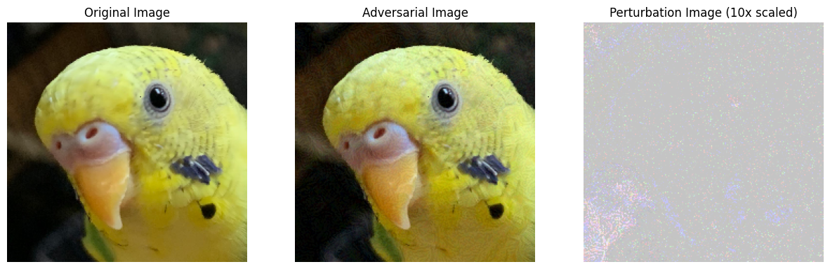
The output adversarial example on burb image using PGD.

Notice how this perturbation image is closer to FGSM than the simple iterative method. The bottom left of this PGD perturbation image shows the pixel different around the bottom left following certain edges, but around the middle it gets sparse.

Let's move forward and try to these techiques to recent CTF challenges.

Applying to recent CTF challenges

In the following two CTF challenges, we will try both the techniques that worked well for us in the previous sections. The navie gradient descent and PGD (following the sign of the gradient). FSGM will be able to generate an adversarial example but will not be able to solve the challenge alone in these cases.

misc / what-a-jpeg-is

ireland

6 solves / 396 points

DiceCTF 2024 Quals

I just want a picture of a god-dang Madagascar cat

nc mc.ax 31373

Let's start by looking at the code (partially shown):

def pytorch_jpeg_compress(img_tensors):
    out_tensors = []
    for img_tensor in img_tensors:
        quality = np.random.randint(50, 90)
        img = Image.fromarray(
            (
                np.clip(img_tensor.cpu().numpy().swapaxes(0, 1).swapaxes(1, 2), 0, 1) * 255
            ).astype(np.uint8)
        )

        with io.BytesIO() as f:
            img.save(f, "JPEG", quality=quality)
            img = Image.open(io.BytesIO(f.getvalue()))

        out_tensor = torch.tensor(
            np.array(img).swapaxes(2, 1).swapaxes(1, 0) / 255,
            device=img_tensor.device,
            dtype=torch.float32,
        )
        out_tensors.append(out_tensor)
    out_tensors = torch.stack(out_tensors)
    return out_tensors

model = ...
np_original = ...

openmybook = T.ToTensor()
normalize = T.Normalize([0.485, 0.456, 0.406], [0.229, 0.224, 0.225])
reading_glasses = T.RandomResizedCrop(384, antialias=True)

for target_id in range(383, 388 + 1):
    breed = model.config.id2label[target_id].split(",")[0]
    inp = input(f"I love cats! My favorite breed is {breed}. Can you show me a picture of one?\n")
    try:
        np_breed = np.frombuffer(base64.standard_b64decode(inp), dtype=np.uint8)
        np_breed = np_breed.reshape(np_original.shape)
        assert np.max(np.abs(np_original.astype(int) - np_breed.astype(int))) < 10
    except:
        print("Sorry I only like cats that look exactly like my cat!", flush=True)
        sys.exit(0)

    for i in range(3):

        image = Image.fromarray(np_breed.astype(np.uint8))
        x = openmybook(image) # ToTensor
        x = x.unsqueeze(0)
        x = pytorch_jpeg_compress(x) # RandomCompress
        x = normalize(x) # ImageNet normalization
        x = reading_glasses(x) # RandomResizedCrop

        with torch.no_grad():
            logits = model(x).logits

        if torch.argmax(logits).item() != target_id:
            print(f"That doesn't look like a {breed}!")
            sys.exit(0)

with open("flag.txt") as f:
    print(f.read())

full code: https://github.com/dicegang/dicectf-quals-2024-challenges/blob/main/misc/what-a-jpeg-is/challenge/challenge.py

A couple of things to note:

The adversarial example needs to be within $9$ pixels of the original image.
The adversarial example needs to be robust to JPEG compression, random crops, and resizing.
We need to generate 5 confident adversarial examples in a row (we can't just get lucky on one).

We already know how we can generate a confident adversarial example through iterative training, methods like FSGM won't work for us here. Generating robust examples will be the real challenge.

We can apply the same augmentations during each iteration loop and apply the gradients slowly until we each the final image. This will create a both a confident and robust adversarial example. The only problem here is that JPEG lossy image encoding is non-differentiable, we can't simply use it out of the box for backward propagation.

After some research it looks like there's already some papers that tackle the same problem:

When I was doing the challenge, I only found the 2017 paper and their codea but the challenge probably could be solved with either (I actually later found out that since quality isn't drastic, it is possible to solve by ignoring the JPEG compression entirely).

Let's try to do both iterative methods (simple gradient following and following the sign of the gradient).

n_iterations = 100
target_output = torch.tensor([383], dtype=torch.long, device=device) # do the same for 383 - 388
eps = 8. / 255. # perturbation size, set lower than needed for rounding errors
bs = 8 # batch size - not really needed, but stabilizes training and improves convergence & consistency of adversarial examples

x = img_original_tensor.clone()
x.requires_grad = True
# helps as each forward pass is different, helps stabilize training
def forward(x):
    x = differentiable_jpeg(x, random.randint(50, 90)) # check the full code
    x = normalize(x)
    x = random_crop(x)
    x = model(x).logits
    return x

for iteration in range(n_iterations):
    optimizer.zero_grad()
    
    logits = forward(torch.cat([x] * bs, dim=0))
    loss = loss_func(logits, torch.cat([target_output] * bs, dim=0))
    loss.backward()

    optimizer.step()

    x.data = torch.clamp(x.data, img_original_tensor - eps, img_original_tensor + eps)

full code: https://github.com/OutWrest/blog-handouts/blob/main/exploring-attacks-1/what-jpeg-is-DiceCTF-2024.ipynb

Output:

Iter: 0    | Loss:  8.5492 | Pred: 281 (54.20%) | min/mean/max diff: 0.00/1.44/3.00
Iter: 10   | Loss:  0.2835 | Pred: 383 (75.32%) | min/mean/max diff: 0.00/5.35/9.00
Iter: 20   | Loss:  0.1862 | Pred: 383 (83.01%) | min/mean/max diff: 0.00/6.11/9.00
Iter: 30   | Loss:  0.1670 | Pred: 383 (84.62%) | min/mean/max diff: 0.00/6.17/9.00
Iter: 40   | Loss:  0.4805 | Pred: 383 (61.85%) | min/mean/max diff: 0.00/6.03/9.00
Iter: 50   | Loss:  0.1488 | Pred: 383 (86.17%) | min/mean/max diff: 0.00/6.14/9.00
Iter: 60   | Loss:  0.0966 | Pred: 383 (90.80%) | min/mean/max diff: 0.00/6.15/9.00
Iter: 70   | Loss:  0.1279 | Pred: 383 (88.00%) | min/mean/max diff: 0.00/6.10/9.00
Iter: 80   | Loss:  0.0514 | Pred: 383 (94.99%) | min/mean/max diff: 0.00/6.08/9.00
Iter: 90   | Loss:  0.0598 | Pred: 383 (94.19%) | min/mean/max diff: 0.00/6.09/9.00

Three images that showcase the adversarial attack.

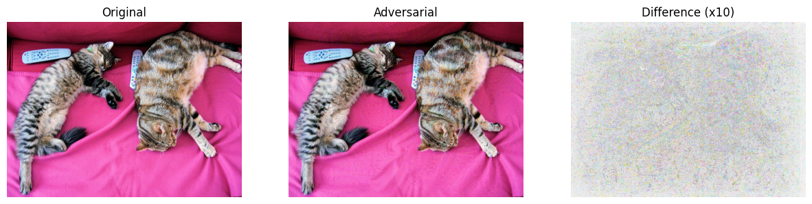
The output adversarial example on provided image using a simple iterative method.

With only $100$ iterations, we easily were able to start making confident adversarial examples. Let's try out PGD and see if we able to get better results.

n_iterations = 100
target_output = torch.tensor([383], dtype=torch.long, device=device) # do the same for 383 - 388
eps = 8. / 255. # perturbation size, set lower than needed for rounding errors
bs = 8 # batch size - not really needed, but stabilizes training and improves convergence & consistency of adversarial examples
alpha = .5 / 255. # step size

x = img_original_tensor.clone()
x.requires_grad = True

loss_func = torch.nn.CrossEntropyLoss()

def forward(x):
    x = differentiable_jpeg(x, random.randint(50, 90))
    x = normalize(x)
    x = random_crop(x)
    x = model(x).logits
    return x

for iteration in range(n_iterations):
    optimizer.zero_grad()
    
    logits = forward(torch.cat([x] * bs, dim=0)) # helps as each forward pass is different, helps stabilize training
    loss = loss_func(logits, torch.cat([target_output] * bs, dim=0))
    
    grad = torch.autograd.grad(loss, x)[0]
    
    x.data = x.data - alpha * torch.sign(grad)
    x.data = torch.clamp(x.data, img_original_tensor - eps, img_original_tensor + eps)

full code: https://github.com/OutWrest/blog-handouts/blob/main/exploring-attacks-1/what-jpeg-is-DiceCTF-2024.ipynb

Output:

Iter: 0    | Loss:  9.8105 | Pred: 281 (48.51%) | min/mean/max diff: 0.00/0.06/1.00
Iter: 10   | Loss:  4.3521 | Pred: 281 (40.86%) | min/mean/max diff: 0.00/0.87/5.00
Iter: 20   | Loss:  5.0837 | Pred: 281 (35.09%) | min/mean/max diff: 0.00/1.42/8.00
Iter: 30   | Loss:  0.6920 | Pred: 383 (50.06%) | min/mean/max diff: 0.00/1.82/9.00
Iter: 40   | Loss:  0.1363 | Pred: 383 (87.25%) | min/mean/max diff: 0.00/2.05/9.00
Iter: 50   | Loss:  0.0625 | Pred: 383 (93.94%) | min/mean/max diff: 0.00/2.22/9.00
Iter: 60   | Loss:  0.0259 | Pred: 383 (97.44%) | min/mean/max diff: 0.00/2.46/9.00
Iter: 70   | Loss:  5.2534 | Pred: 281 (27.16%) | min/mean/max diff: 0.00/2.70/9.00
Iter: 80   | Loss:  0.0133 | Pred: 383 (98.68%) | min/mean/max diff: 0.00/2.89/9.00
Iter: 90   | Loss:  0.0045 | Pred: 383 (99.55%) | min/mean/max diff: 0.00/3.13/9.00

PDG is able generate more confident examples at a lesser perturbation difference. Please check out the full code listed above, it should be all reproducible.

The output adversarial example on provided image using PGD.

To solve the rest the challenge, we just need to do this 5 more times and try them out remote machine. I do not have the full solve code here but you can easily extend the scripts I have provided to do so.

misc / i-hate-anime-girls

segal

6 solves / 396 points

osu!gaming CTF 2024

osu! players love their anime girls. But I HATE anime girls. So much so that I trained a neural network to filter my map backgrounds. But tbh, I really want to pp farm hitorigoto and my map filter won't let me. Can you fool it?

nc chal.osugaming.lol 7274

This challenge comes with 3 different files, hitorigoto.png, model.pt, and server.py. Let's explore the code first to figure out how to get the flag.

model = resnet18()
model.fc = nn.Linear(model.fc.in_features, 1)
model.load_state_dict(torch.load("model.pt"))

resize = T.Resize((224, 224), antialias=None)
to_tensor = T.ToTensor()
normalize = T.Normalize([0.485, 0.456, 0.406], [0.229, 0.224, 0.225])

original = np.array(Image.open("hitorigoto.png"))

inp = input(f"Enter a base64 encoded image.\n")
try:
    img = np.frombuffer(base64.standard_b64decode(inp), dtype=np.uint8)
    img = img.reshape(original.shape)
    assert np.max(np.abs(original.astype(np.int32) - img.astype(np.int32))) <= 8
except:
    print("That doesn't look like hitorigoto!")
    sys.exit(0)

image = Image.fromarray(img)
x = normalize(resize(to_tensor(image)).unsqueeze(0))
with torch.no_grad():
    y = torch.sigmoid(model(x))

if y < 0.5:
    print("That's obviously an anime girl.")
    sys.exit(0)
elif y < 0.825:
    print("I'm not fully convinced that's not an anime girl.")
    sys.exit(0)

with open("flag.txt") as f:
    print("Surely that's not an anime girl.")
    print(f.read())

full code: https://drive.google.com/file/d/1qqJ2xrlrvppz50bjAzmfhpX66Y-UkqnM/view

The whole point of this challenge seems to be able to create a confident (>82.5% confidence) adversarial example from the given image that is able to be resistant against the resizing. We already know how to do this, but this challenge posed a problem for me initially. I was getting very inconsistent results. I found out the challenge author left out the .eval() in the code. This left the current model in training mode. For us, this just means that it will be harder to generate adversarial example because the batch normalization layers won't be applied to our input.

Let's try the same two methods in the previous challenge on this one.

n_iterations = 1250
eps = 7. / 255.
bs = 32 # not needed

x = img_original_tensor.clone().detach().requires_grad_(True)

# made use of lr_scheduler to reduce the learning rate when the loss stops decreasing
# this helps model converge as this problem is hard to optimize
optimizer = torch.optim.Adam([x], lr=5e-1) # we will only optimize the input image
lr_scheduler = torch.optim.lr_scheduler.ReduceLROnPlateau(optimizer, patience=50, verbose=True, factor=0.5)
loss_func = nn.BCEWithLogitsLoss()

def forward(x):
    x = resize(x)
    x = normalize(x)
    x = model(x)
    return x

for iteration in range(n_iterations):
    optimizer.zero_grad()

    logits = forward(torch.cat([x] * bs, dim=0)) # bs not needed
    loss = loss_func(logits, torch.ones_like(logits)) # maximize the output of the model
    loss.backward()

    optimizer.step()

    lr_scheduler.step(loss)

    x.data = torch.clamp(x.data, img_original_tensor - eps, img_original_tensor + eps)

full code: https://github.com/OutWrest/blog-handouts/blob/main/exploring-attacks-1/i-hate-anime-girls-osugaming-2024.ipynb

Output:

Iter: 0    | Loss:  2.0104 | Pred:  0.1339 | min/mean/max diff: 0.00/4.80/8.00
Iter: 62   | Loss:  0.8145 | Pred:  0.4429 | min/mean/max diff: 0.00/4.46/8.00
Iter: 124  | Loss:  0.7141 | Pred:  0.4896 | min/mean/max diff: 0.00/4.50/8.00
Iter: 186  | Loss:  0.4650 | Pred:  0.6282 | min/mean/max diff: 0.00/4.40/8.00
Iter: 248  | Loss:  0.4427 | Pred:  0.6423 | min/mean/max diff: 0.00/4.45/8.00
Iter: 310  | Loss:  0.3205 | Pred:  0.7258 | min/mean/max diff: 0.00/4.26/8.00
Iter: 372  | Loss:  0.3281 | Pred:  0.7203 | min/mean/max diff: 0.00/4.12/8.00
Iter: 434  | Loss:  0.2920 | Pred:  0.7468 | min/mean/max diff: 0.00/3.94/8.00
Iter: 496  | Loss:  0.2534 | Pred:  0.7762 | min/mean/max diff: 0.00/3.69/8.00
Iter: 558  | Loss:  0.1844 | Pred:  0.8316 | min/mean/max diff: 0.00/3.61/8.00
Iter: 620  | Loss:  0.1768 | Pred:  0.8380 | min/mean/max diff: 0.00/3.63/8.00
Iter: 682  | Loss:  0.1810 | Pred:  0.8344 | min/mean/max diff: 0.00/3.67/8.00
Iter: 744  | Loss:  0.1501 | Pred:  0.8606 | min/mean/max diff: 0.00/3.66/8.00
Iter: 806  | Loss:  0.1472 | Pred:  0.8631 | min/mean/max diff: 0.00/3.66/8.00
Iter: 868  | Loss:  0.1463 | Pred:  0.8639 | min/mean/max diff: 0.00/3.68/7.00
Iter: 930  | Loss:  0.1309 | Pred:  0.8773 | min/mean/max diff: 0.00/3.68/8.00
Iter: 992  | Loss:  0.1298 | Pred:  0.8783 | min/mean/max diff: 0.00/3.67/8.00
Iter: 1054 | Loss:  0.1285 | Pred:  0.8794 | min/mean/max diff: 0.00/3.68/8.00
Iter: 1116 | Loss:  0.1282 | Pred:  0.8796 | min/mean/max diff: 0.00/3.70/8.00
Iter: 1178 | Loss:  0.1210 | Pred:  0.8860 | min/mean/max diff: 0.00/3.70/7.00
Iter: 1240 | Loss:  0.1207 | Pred:  0.8863 | min/mean/max diff: 0.00/3.70/7.00

We had to use some tricks to generate an examples that is able to be confident enough for the flag. I had to apply a learning rate scheduler that would reduce the step size by half if it doesn't improve after 50 iterations.

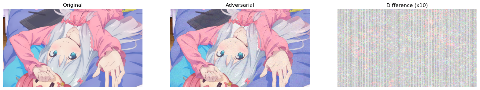
The output adversarial example on provided image using a simple iterative method.

The difference map shows something very interesting with vertical lines spread throughout. I think this is an artifact of optimizing before the resizing operation. Let's try the PGD and see if it does better.

n_iterations = 2000
eps = 7. / 255.
bs = 32 # not needed
alpha = .1

iters_since_improvement = 0
max_iters_since_improvement = 100
best_loss = float('inf')

x = img_original_tensor.clone().detach().requires_grad_(True)

loss_func = nn.BCEWithLogitsLoss()

def forward(x):
    x = resize(x)
    x = normalize(x)
    x = model(x)
    return x

for iteration in range(n_iterations):
    model.zero_grad() # this is the fix for the author's mistake

    logits = forward(torch.cat([x] * bs, dim=0)) # bs not needed
    loss = loss_func(logits, torch.ones_like(logits)) # maximize the output of the model

    grad = torch.autograd.grad(loss, x)[0]
    x.data = x.data - alpha * torch.sign(grad)

    x.data = torch.clamp(x.data, img_original_tensor - eps, img_original_tensor + eps)

    if loss.item() < best_loss - 0.05:
        best_loss = loss.item()
        iters_since_improvement = 0
    else:
        iters_since_improvement += 1
        if iters_since_improvement >= max_iters_since_improvement:
            alpha /= 1.5
            iters_since_improvement = 0
            print(f"Reducing alpha to {alpha}")

full code: https://github.com/OutWrest/blog-handouts/blob/main/exploring-attacks-1/i-hate-anime-girls-osugaming-2024.ipynb

Output:

Iter: 0    | Loss:  2.0104 | Pred:  0.1339 | min/mean/max diff: 0.00/4.80/8.00
Iter: 100  | Loss:  2.0053 | Pred:  0.1346 | min/mean/max diff: 0.00/4.80/8.00
Reducing alpha to 0.06666666666666667
Iter: 200  | Loss:  1.9217 | Pred:  0.1464 | min/mean/max diff: 0.00/4.79/8.00
Reducing alpha to 0.044444444444444446
Iter: 300  | Loss:  1.8906 | Pred:  0.1510 | min/mean/max diff: 0.00/4.23/8.00
Reducing alpha to 0.02962962962962963
Iter: 400  | Loss:  1.8724 | Pred:  0.1538 | min/mean/max diff: 0.00/3.31/7.00
Iter: 500  | Loss:  1.5570 | Pred:  0.2108 | min/mean/max diff: 0.00/3.32/8.00
Reducing alpha to 0.019753086419753086
Iter: 600  | Loss:  1.4528 | Pred:  0.2339 | min/mean/max diff: 0.00/3.20/8.00
Iter: 700  | Loss:  1.5776 | Pred:  0.2065 | min/mean/max diff: 0.00/3.20/8.00
Reducing alpha to 0.01316872427983539
Iter: 800  | Loss:  1.2085 | Pred:  0.2986 | min/mean/max diff: 0.00/2.97/8.00
Reducing alpha to 0.008779149519890261
Iter: 900  | Loss:  0.9222 | Pred:  0.3976 | min/mean/max diff: 0.00/2.87/8.00
Reducing alpha to 0.005852766346593507
Iter: 1000 | Loss:  0.6689 | Pred:  0.5123 | min/mean/max diff: 0.00/2.97/8.00
Iter: 1100 | Loss:  0.5700 | Pred:  0.5655 | min/mean/max diff: 0.00/3.03/8.00
Reducing alpha to 0.003901844231062338
Iter: 1200 | Loss:  0.4041 | Pred:  0.6676 | min/mean/max diff: 0.00/3.21/8.00
Reducing alpha to 0.002601229487374892
Iter: 1300 | Loss:  0.4183 | Pred:  0.6581 | min/mean/max diff: 0.00/3.25/7.00
Iter: 1400 | Loss:  0.3224 | Pred:  0.7244 | min/mean/max diff: 0.00/3.19/7.00
Reducing alpha to 0.0017341529915832611
Iter: 1500 | Loss:  0.2673 | Pred:  0.7654 | min/mean/max diff: 0.00/3.22/7.00
Reducing alpha to 0.0011561019943888407
Iter: 1600 | Loss:  0.2352 | Pred:  0.7904 | min/mean/max diff: 0.00/3.25/7.00
Reducing alpha to 0.0007707346629258938
Iter: 1700 | Loss:  0.2144 | Pred:  0.8070 | min/mean/max diff: 0.00/3.28/7.00
Reducing alpha to 0.0005138231086172625
Iter: 1800 | Loss:  0.2014 | Pred:  0.8176 | min/mean/max diff: 0.00/3.29/7.00
Reducing alpha to 0.000342548739078175
Iter: 1900 | Loss:  0.1925 | Pred:  0.8249 | min/mean/max diff: 0.00/3.30/7.00
Reducing alpha to 0.00022836582605211667

I wasn't able to generate another example that does better than the previous method in terms of confidence using PGD. But it should be enough to be used to solve the challenge.

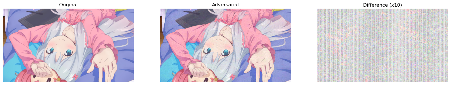
The output adversarial example on provided image using PGD.

Conclusion

In this exploration of a few different adversarial attacks on CNNs, we learned about some widely used practical techiques, specifically in context of solving CTF challenges. I really hope that conveyed these ideas clearly and I would strongly encourage you to go through the code repository linked to get a clearer idea about how to apply these methods.

While brief, I wanted to show some real examples from CTF challenges that used similar ideas. I think we'll probably see more CTFs creating AI/ML focused challenges. Feel free to reach out to me through discord if you have any questions.